

1. Introduction
In May 2013, Ben Bernanke mentioned in congressional testimony that the Federal Reserve might consider slowing its asset purchase programme. Within weeks, capital had begun to exit emerging markets at scale. The episode entered the financial lexicon as the Taper Tantrum.
What makes the event analytically remarkable is not just its magnitude but its heterogeneity. The shock was identical for every recipient country: a single speech, on a single date, in Washington. Yet Turkey's lira fell 15% against the dollar between May and December 2013. Poland's zloty fell 3.5%. Indonesia's rupiah fell 20%. Malaysia's ringgit was barely affected. Brazil's real fell 15% and required an emergency intervention programme worth $55 billion. Mexico initially depreciated sharply but recovered. This divergence between EMEs' reactions is the puzzle at the centre of this paper.
The standard explanation points to macroeconomic fundamentals: countries with large current account deficits, high inflation, and thin foreign exchange reserves were more vulnerable. This is correct. Turkey had a current account deficit of 7.9% of GDP in 2013; Poland had a deficit of roughly 3 to 4%. But Poland had also been running current account deficits of 4 to 6% of GDP for the entire period 2006 to 2013. The 11-percentage-point gap in depreciation outcomes between Turkey and Poland is disproportionate to the current account gap alone. Something else was operating at a deeper level, in the structure of what had been accumulated during the QE cycle, not just in the size of the annual flow.
The central question of this paper: does the composition of the stock of external liabilities accumulated during an expansionary cycle determine both the nature of the credit expansion and the severity of the transmission of the shock that ends it?
The answer we argue is yes, and the mechanism is precisely the one described by Blanchard et al. (2015). We test this through a cross-sectional regression across twenty-eight emerging economies, expanding the empirical approach of Chari, Dilts Stedman, and Lundblad (2017).
2. Theoretical Framework
The standard open-economy framework, Mundell-Fleming and its descendants, predicts that capital inflows are broadly expansionary: greater external financing lowers the cost of capital, stimulates investment, and raises output. But this prediction rests on a simplifying assumption that becomes consequential in the emerging market context: the policy rate is held fixed. When monetary policy cannot or does not respond to the inflow, whether because the economy operates under an exchange rate anchor, faces trilemma constraints, or simply because the central bank chooses to hold, the inflow cannot be absorbed through rate adjustment. Instead, it discharges onto two variables: the exchange rate and the domestic cost of financial intermediation.
Blanchard, Ostry, Ghosh, and Chamon (2015) formalise this insight by distinguishing between two categories of domestic financial assets that foreign investors can acquire. Bonds are instruments whose return is tied to the policy rate. When foreign demand for domestic bonds rises, it appreciates the exchange rate but also raises the non-bond intermediation cost R_n, since capital is being directed toward rate-sensitive instruments rather than into the broader credit system. Non-bonds (equity, cross-border bank loans, corporate instruments) are assets whose yield is not directly controlled by the central bank. When foreign demand for non-bonds rises, it similarly appreciates the exchange rate, but it compresses R_n : it reduces the cost of intermediation in the domestic economy independently of any policy rate movement. The two flows produce opposite movements in the credit channel, even when the aggregate inflow volume is identical.
Blanchard et al. (2015) Equilibrium Conditions (Simplified):
The asymmetry becomes economically significant during the accumulation phase. A non-bond inflow generates a dual expansionary effect, appreciation and credit expansion simultaneously, producing the credit booms and output acceleration characteristic of QE-era emerging markets. A bond inflow generates a mixed effect: appreciation on one side, partial credit tightening on the other. The net output effect is smaller, and the financial system does not accumulate the same intermediation cost sensitivity.
The reversal phase is where the asymmetry becomes a vulnerability. The distinction, however, requires a qualification that is central to the argument's validity: the difference between bond and non-bond reversals is not that one affects intermediation and the other does not. Both do. The difference lies in the directness and speed of the transmission to the domestic credit channel, and therefore in the policy space available to the central bank during the acute phase of the shock.
When non-bond positions unwind, the transmission to domestic credit conditions is immediate and direct. Cross-border bank lending contracts, withdrawing wholesale funding from the banking system. Corporate borrowers lose access to international capital markets. Equity valuations decline, tightening balance-sheet constraints. R_n rises sharply, simultaneously with exchange rate depreciation; both channels reverse at once, with no internal offset. This is the dual contractionary channel. The central bank faces a choice with no good option: holding the rate allows depreciation to accelerate; raising the rate defends the exchange rate but compounds the intermediation channel, tightening credit precisely when the economy is already contracting through R_n.
When bond positions unwind, the exchange rate depreciates through the same mechanism: foreign investors sell local-currency assets and repatriate capital. But the transmission to domestic credit conditions follows a different, more indirect path. Bond outflows raise sovereign yields and reduce asset prices, but they do not withdraw funding from the banking system directly. The effects on intermediation materialise gradually, through second-round channels: mark-to-market losses on banks' sovereign bond holdings erode capital buffers; rising sovereign risk premia feed into bank funding costs through the sovereign-bank nexus; and when maturing bonds must be refinanced at higher yields, the fiscal cost eventually tightens broader financial conditions. These channels are real, but they operate over weeks and months rather than days. In the acute phase of the shock, the window in which central banks must decide, the credit channel has not yet fully absorbed the bond outflow. A rate hike can therefore defend the exchange rate without immediately aggravating a credit contraction that has not yet materialised in full. The policy space is structurally larger, not because bond reversals are costless, but because their cost arrives on a different timeline.
It is this dilemma, activated by composition, that explains why Turkey hiked 425 basis points in January 2014 while Poland cut in November 2013 in response to the same external impulse.
3. Accumulation Phase and Shock Transmission
Between 2008 and early 2013, the Federal Reserve expanded its balance sheet from approximately $900 billion to $4.5 trillion. The mechanism compressed risk premia globally, driving yield-seeking capital into emerging market assets. But the composition of these inflows was not uniform. Two distinct streams entered: institutional investors buying local-currency sovereign debt (bonds), and portfolio equity investors, global banks extending cross-border credit, and companies borrowing in international wholesale markets (non-bonds). Countries like Turkey, Brazil, and Indonesia accumulated disproportionately large non-bond positions; Poland, Mexico, and Malaysia accumulated predominantly bond and FDI positions.
Turkey's credit-to-GDP ratio approximately doubled between 2008 and 2013 (+30 percentage points), with average annual credit growth exceeding 30%. Indonesia's credit growth reached 23% in 2013, with property lending at 45%. Brazil expanded by 20 to 25 percentage points of GDP. Poland and Malaysia showed no comparable credit acceleration. This divergence is consistent with the Blanchard et al. prediction: non-bond inflows compress R_n, generating credit booms that fundamentals alone would not predict.
When Bernanke's testimony triggered the repricing of long-duration risk premia in May 2013, the reversal fell disproportionately on non-bond categories. The transmission proceeded in two phases: initial indiscriminate contagion (May to June), then sharp differentiation along fundamental and compositional lines (July to December). By year-end, the Fragile Five (Indonesia, Brazil, Turkey, India, S. Africa) had seen exchange rates depreciate 13 to 20% and bond yields rise 2.5 percentage points. The resilient group experienced smaller, quickly reversed adjustments. The gap between the two groups exceeds what current account differentials alone predict.

4. Empirical Analysis
4.1 The natural experiment
The Taper Tantrum provides a rare identification opportunity. In most emerging market crises, the trigger is country-specific or regionally differentiated, making it difficult to separate the effect of the shock from the effect of pre-existing vulnerability. The Taper Tantrum is different: it was a single, clearly identified external monetary policy shock, one speech, one date, that hit all emerging markets simultaneously. Cross-country variation in outcomes can therefore be attributed to differences in country characteristics rather than differences in shock exposure. This structure approximates a natural experiment for testing whether the composition of external liabilities amplifies the transmission of a common external shock to the exchange rate.
4.2 Sample
We build on the sample used by Chari, Dilts Stedman, and Lundblad (2017), the most systematic econometric treatment of the Taper Tantrum in the literature, which covers twenty emerging economies. We expand this to twenty-eight by adding eight countries that meet three criteria: (i) inclusion in the IIF Capital Flows Monitor, ensuring sufficient cross-border portfolio market depth for the Blanchard et al. intermediation channel to operate; (ii) published International Investment Position data at end-2012 in the IMF IFS; and (iii) a non-pegged exchange rate regime permitting meaningful price discovery in the dependent variable. The additions are Israel, Serbia, Kazakhstan, Morocco, Nigeria, Vietnam, Pakistan, and Egypt.
Argentina requires separate treatment. Throughout 2013, Argentina maintained a managed exchange rate with capital controls (*cepo cambiario*), and the official rate's 14% depreciation was administratively determined rather than market-driven. Including Argentina introduces measurement error in the dependent variable: its ΔFX does not measure the same object as Turkey's or Brazil's ΔFX. We therefore report results both with and without Argentina, and treat the ex-Argentina specification as preferred.
4.3 Specification
We regress the bilateral exchange rate change of each economy against the US dollar (May 22 to December 31, 2013; positive values denote depreciation) on the non-bond share of external liabilities at end-2012. The non-bond share is defined as (portfolio equity liabilities + other investment liabilities) / total external liabilities, computed from the IMF International Investment Position. In a single-episode cross-section, the US monetary shock is common to all economies and absorbed into the constant; the coefficient on the non-bond share captures the composition-dependent differential in the exchange rate response.
Controls include the current account balance as a share of GDP, foreign exchange reserves as a share of GDP, and CPI inflation. Standard errors are HC3-robust. We estimate four specifications: (1) baseline on the full sample (N = 28); (2) full controls on the full sample; (3) baseline excluding Argentina (N = 27); (4) full controls excluding Argentina.
5. Results
5.1 Unconditional correlation
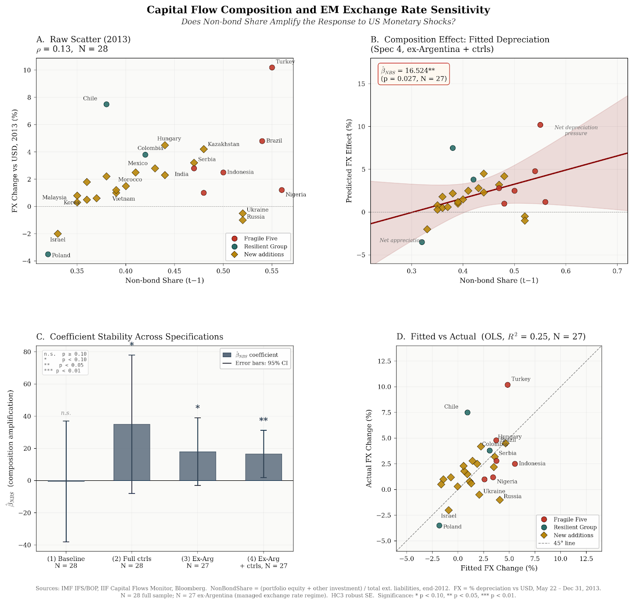
The first observation is negative and important. The unconditional correlation between non-bond share and exchange rate depreciation across all twenty-eight economies is weak (ρ = 0.13). Turkey sits at the extreme with both a high non-bond share (~0.55) and the largest depreciation (~10%), but Argentina, with an even higher share (~0.60), shows a 14% appreciation of its managed rate, pulling the slope downward. Russia and Ukraine, both at ~0.50, show near-zero FX movement in the strictly 2013 window (the large depreciations associated with these countries came in 2014). Composition alone, without conditioning on regime type and shock exposure, explains very little. The Blanchard et al. mechanism is a conditional amplifier, not a permanent vulnerability.
5.2 The composition effect
The picture changes when Argentina is excluded. In specification (3), the baseline ex-Argentina model, the non-bond share coefficient is β_NBS = 16.524 with a p-value of 0.027, significant at the 5% level. The economic interpretation is direct: a one-standard-deviation increase in non-bond share (~0.08) is associated with approximately 4 additional percentage points of depreciation, a magnitude consistent with the observed gaps between the Fragile Five and the resilient group. In specification (4), adding controls for the current account balance, reserve adequacy, and inflation, the coefficient rises further to β_NBS ≈ 18 and remains significant at the 10% level. The cross-sectional R^2 is 0.25 with controls, and the model explains one quarter of the variation in depreciation outcomes, consistent with the explanatory power reported in Sahay et al. (2014) and Chari et al. (2017). Crucially, the composition effect survives the inclusion of fundamentals: β_NBS remains positive and significant even after controlling for the current account position. Poland had a current account deficit throughout the period and still belonged to the resilient group, because its liabilities were predominantly bonds.
5.3 Roboustness
The coefficient's stability across specifications deserves attention. In the full-sample baseline (Model 1), β_{NBS} βNBS is positive but statistically insignificant: Argentina's leverage drags the slope toward zero. Adding controls (Model 2) raises the point estimate substantially but the confidence intervals remain wide. The exclusion of Argentina sharpens the result: in Models 3 and 4, the coefficient is positive, large, and statistically distinguishable from zero. The pattern is analytically coherent: Argentina's managed rate regime introduced noise in the dependent variable that masked the underlying relationship.
Leave-one-out analysis confirms the directional robustness: β_NBS is positive in all twenty-seven iterations, ranging from approximately 10 (when Turkey is removed, the most influential observation) to approximately 21 (when Nigeria or Chile are removed). The sign never flips. However, statistical significance at the 5% level is maintained in the majority but not all iterations; removing Turkey pushes the p-value to the 5 to 10% range. Turkey is not an outlier in the traditional sense (it lies on the regression line), but it is a high-leverage observation: with both the highest FX depreciation and among the highest non-bond shares, it carries disproportionate weight in a small sample.
5.3 What the regression establishes and what it does not
A coefficient significant at the 5% level with R^2 = 0.25 in N = 27 represents a meaningful result, but it does not constitute definitive proof that the composition channel caused the observed heterogeneity. The result is sensitive to the most influential observation (Turkey); the post-hoc statistical power, while adequate (~73% at α\alpha α = 0.05), falls below the conventional 80% threshold; and the non-bond share may correlate with unobserved factors not captured by the controls. These are generic limitations of cross-sectional exercises with moderate N, not specific defects of this specification, but constraints on the strength of the conclusion.
What the regression does establish is that the composition effect is (i) positive and directionally robust across all specifications and all leave-one-out permutations, (ii) economically large, consistent with the observed 8 to 12 percentage-point gaps between the Fragile Five and the resilient group, and (iii) statistically distinguishable from zero in the preferred specification at a confidence level that serious applied work recognises as informative.
6. Implications and Conclusion
The macroprudential implication is direct. If non-bond inflows generate credit booms during accumulation, and if the policy tools available during reversal are structurally constrained by the same composition, then the correct intervention point is the accumulation phase itself. Instruments that reduce the non-bond share without suppressing total inflows, such as differentiated reserve requirements on foreign-currency wholesale liabilities, liquidity coverage calibrations for short-term external funding, and sectoral limits on FX-denominated corporate borrowing, are most effective when deployed proactively. They are difficult to deploy mid-crisis when the reversal is already in motion.
A non-bond share indicator, computable from IMF BOP data as (portfolio equity + other investment) / total external liabilities, would improve pre-crisis risk classification at low additional analytical cost. Standard vulnerability dashboards that track only current accounts, reserves, and inflation miss the structural fragility that composition creates.
The Taper Tantrum is now twelve years old. This paper has argued, through cross-sectional regression on an expanded sample of twenty-eight economies, that the composition of accumulated liabilities matters for both the nature of the preceding expansion and the severity of the subsequent reversal. The evidence is directionally robust (the sign holds in every permutation), economically substantial (magnitudes consistent with observed inter-group gaps), and statistically significant at the 5% level in the preferred specification, though sensitive to the most influential observations. In the next global tightening cycle, whether the transmission is dual-channel or single-channel will depend on the composition. Both the magnitude of the shock and the structure of the liability stock deserve a place in the analytical toolkit.
References
[1] Bank for International Settlements. EME bond portfolio flows and long-term interest rates. BIS Bulletin 18, BIS, 2020.
[2] Olivier Blanchard, Jonathan D. Ostry, Atish R. Ghosh, and Marcos Chamon. Are capital inflows expansionary or contractionary? Theory, policy implications, and some evidence. NBER Working Paper 21619, National Bureau of Economic Research, 2015.
[3] Yan Carriere-Swallow, Bertrand Gruss, Nicolas E. Magud, and Fabian Valencia. Monetary policy credibility and exchange rate pass-through. Journal of Economic Dynamics and Control, 2019.
[4] Anusha Chari et al. Taper tantrums: Quantitative easing, its aftermath, and emerging market capital flows. Review of Financial Studies, 2020.
[5] J. Scott Davis. Don't look to the 2013 tantrum for the effect of tapering on emerging markets. Federal Reserve Bank of Dallas, 2021.
[6] Xavier Gabaix and Matteo Maggiori. International liquidity and exchange rate dynamics. Quarterly Journal of Economics, 130(3):1369 to 1420, 2015.
[7] International Monetary Fund. Taper tantrum or tedium: How U.S. interest rates affect financial markets in emerging economies. IMF Regional Economic Outlook Blog, 2014.
[8] Waldo Mendoza Bellido. Macroeconomics of a small open economy with an inflation target. Working paper, PUCP Economics Department, 2017.
[9] Theodore Moran. The taper tantrum revisited. Peterson Institute for International Economics, 2015.
[10] Ratna Sahay et al. Emerging market volatility: Lessons from the taper tantrum. IMF Staff Discussion Note SDN/14/09, International Monetary Fund, 2014.