

1. Introduction
On April 15th 2015, John Brian Taylor, renowned American economist and professor at Stanford University, after giving out a brief review of Fed’s monetary policy strategy from 1950s to contemporary times, stated : "This short history demonstrates that shifts toward and away from steady predictable monetary policy have made a great deal of difference for the performance of the economy, just as basic macroeconomic theory tells us... The implication of this experience is clear: monetary policy should re-normalize in the sense of transitioning to a predictable rule-like strategy for the instruments of policy". By quoting a rule-like strategy, the economist refers to his widely discussed Taylor Rule, a simple equation connecting the FOMC’s (i.e. Federal Open Market Committee) target for the federal funds rate, namely the interest rate at which banks make overnight loans to each other, to the current state of the economy. Taylor introduced this numerical formula in a 1993 paper, laying foundations for a revolutionary view of monetary policy, based on empirical econometric research applied to operational decision-making.
2. The Taylor Rule: Catalyst for the Rule-Based Approach
2.1. Equation and Elements of the Original Taylor Rule
The analytical rule proposed by the Newyorkese economist consists of:
- r is the nominal federal funds rate, the output of the equation, while r* is the standard interest rate, set at 2% as an approximation of the GDP growth trend rate, as taught by common neoclassical growth models. Hence, this precise estimate served as long run "equilibrium" rate;
- i represents the inflation rate measured through the GDP deflator, which accounts for total inflation of an entire economy, thus it also considers more volatile elements such as food and energy. The target inflation rate is i ∗ , also set at 2%. This choice was driven by the Zero Lower Bound (ZLB) problem. At the time,the ZLB consisted of the actual limit underneath which lowering rates had no expansionary effects anymore, identified as 0%. Nowadays, instead, economists tolerate even slight negative rates and the limit is defined as Expected Lower Bound (ELB). Back to the ZLB, imagine this: if target inflation rate was set at 0%, then the Fed would have had no room to provide extra economic stimulus by lowering policy rates whenever needed, easily incurring into exceeding the target. Instead, with a target rate of 2%, a buffer zone for stimulus was guaranteed;
- (y − y∗) corresponds to the percentage delta of the real GDP from the target one. The target GDP consists of the potential output achieved when capital and labor are fully exploited. Hence, this delta is also known as output gap. At the time, Taylor employed a 2.2% growth trend as target GDP for the model, based on GDP growth recorded from 1984.
Therefore, through his very first original rule, Taylor would predict that the FOMC would have increased the fed funds rate by 0.5% for every excessive percentage point of the inflation rate compared to the target one, same goes for every percentage point of the ouput gap. Reasoning accordingly, the real policy rate consequence of an inflation rate fully aligned with the target one and a null output gap would be exactly 2%, namely the long run "equilibrium" rate.
Also in his 1993 paper, Taylor stated how this rule was able to describe pretty accurately FOMC decisions in the 1987-1992 interval, with the only exception of a significant deviation in October 1987, when the Fed had to react to the Black Monday, a severe and sudden stock market crash, by proactively easing rates. This can be undoubtedly observed in Figure 1:
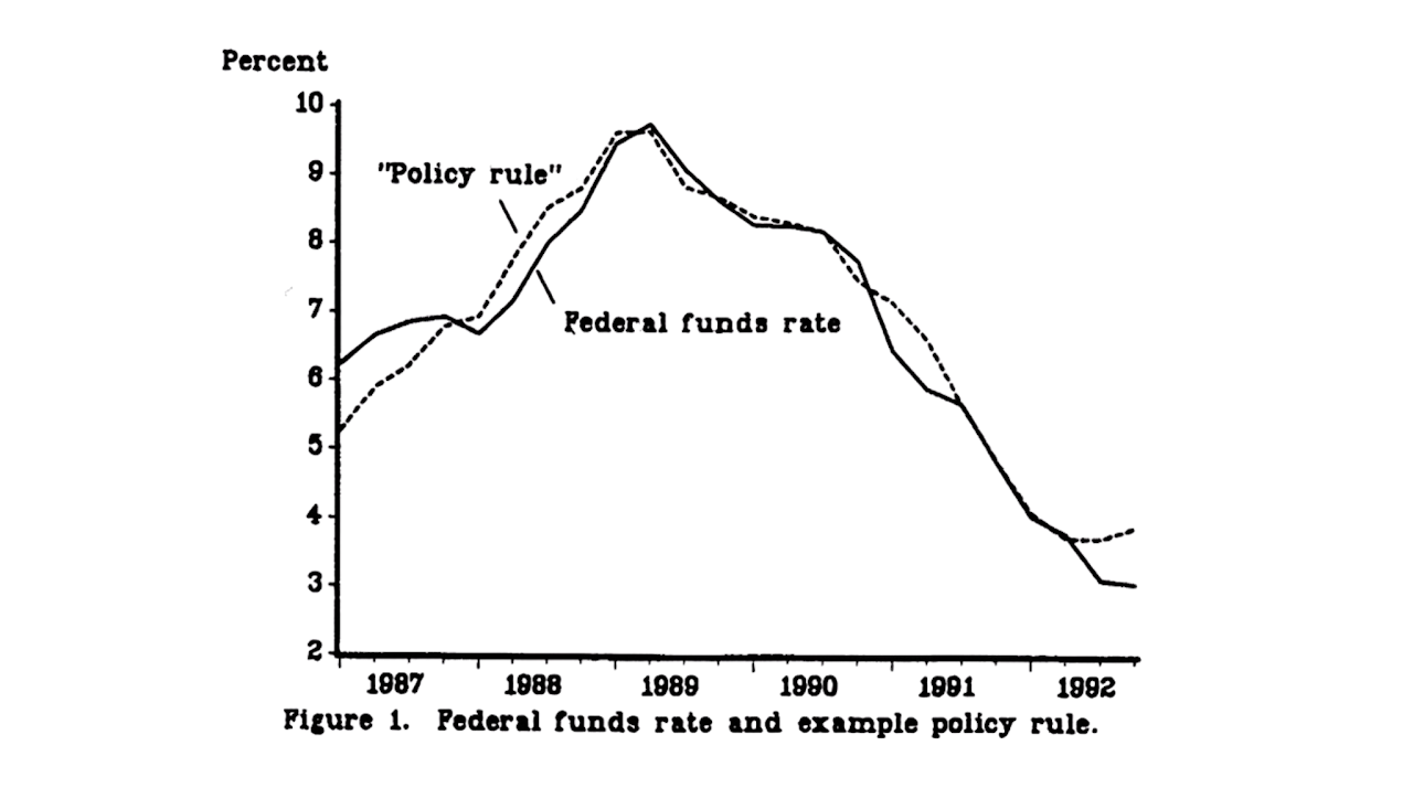
Figure 1: Comparison between actual federal funds rates and policy rates estimated by the original Taylor Rule throughout 1987-1992
2.2. Evolution of Taylor’s Thought
Now, despite claiming that his rule could explain decisions made by the FOMC in a quite thorough way, Taylor did not initially believe that monetary policy strategy needed to actually follow a strict rule-based approach, as his research was mostly aimed at delivering a general headline for policy rates. This made absolute sense, since it would have been limiting to think that a simple analytical equation could incorporate all factors characterizing complex macroeconomic environments, even if less intricate and interconnected compared to nowadays.
As time passed by, however, Taylor’s point of view changed drastically: firstly, he claimed that in the run from 2003 to mid-2005 rates were kept abundantly low compared to what his rule would’ve prescribed, and that this estrangement from the rule-based approach was one of the catalysts which led to the housing bubble and the Great Financial Crisis.
Afterwards, he also heavily criticized the discretionary approach which reigned post-GFC, characterized by the adoption of unconventional measures such as Quantitative Easing (QE). In his 2015 intervention, he argued.
"This deviation from rules-based monetary policy went beyond the United States, as first pointed out by researchers at the OECD (i.e. Organisation for Economic Co-operation and Development), and is now obvious to any observer. Central banks followed each other down through extra low interest rates in 2003-2005 and more recently through quantitative easing. QE in the US was followed by QE in Japan and by QE in the Eurozone with exchange rates moving as expected in each case. Researchers at the BIS showed the deviation went beyond OECD and called it the Global Great Deviation... Complaints about spillover and pleas for coordination grew. NICE (Non-Inflationary Consistently Expansionary) ended in both senses of the word. World monetary policy now seems to have moved into a strategy-free zone".
3. Bernanke’s Updated Rule in a Brand New Environment
3.1. Adaptation, Not Rejection
Taylor’s criticism did not go unnoticed. After the GFC, the global macroeconomic landscape became exponentially more delicate and monetary economists had to adapt accordingly. In defense of the new strategies and in opposition to Taylor’s rhetoric, Ben Bernanke, former President of the Federal Reserve, intervened directly, not to dismiss the Taylor Rule, but to refine it.
In his 2015 Brookings article, Bernanke engaged with Taylor’s claims on their own terms. Rather than rejecting the rule-based framework, he proposed a modified Taylor Rule, namely an updated version of the same equation, arguing that it provided a more accurate description of sensible monetary policy and, crucially, a better benchmark for evaluating the Fed’s actions in a post-crisis world. His modification was not a refusal of Taylor’s logic, but an adaptation to two key realities: the Fed’s actual operational framework and the unprecedented nature of the Effective Lower Bound (ELB).
The financial crisis had exposed a critical vulnerability in the original Taylor Rule: the Zero Lower Bound (ZLB). As John Taylor himself noted, the ZLB represented the threshold below which nominal interest rates could not be pushed, as economic agents would theoretically prefer to keep cash yielding 0% rather than paying to hold deposits. The 2008 crisis demonstrated that when policy rates hit this bound, central banks lost their primary tool for stimulating the economy. This constraint forced monetary policymakers into what Taylor defined a "strategy-free zone" of unconventional measures like QE and forward guidance. We will come back on these tools in one of the next paragraphs.
Bernanke’s response was to acknowledge that the bound was not absolute, but effective. The distinction between ZLB and ELB is crucial: while the ZLB was a theoretical absolute at 0%, the ELB recognizes that rates can technically go slightly negative (as seen in Europe and Japan), but there remains a practical floor below which further cuts become not only ineffective, but even counterproductive, leading to liquidity accumulation and financial disintermediation.
3.2. Bernanke’s Modified Rule: Equation and Elements
Bernanke’s updated framework can be expressed as an analytical equation, just like Taylor’s original:
Where:
- r is the nominal federal funds rate, again the output of the equation, also r∗ remains the real equilibrium rate, though Bernanke acknowledged that in the post-crisis environment this had likely fallen significantly below Taylor’s original 2% assumption;
- i^core represents the core PCE inflation rate, not the GDP deflator. This is the most significant technical change. While Taylor’s original rule used the GDP deflator, namely a broad index including capital goods and government spending but excluding imports, Bernanke argues that this is not what the FOMC actually targets. In practice, the Fed’s preferred measure is the rate of change in consumer prices, specifically the deflator for personal consumption expenditures (PCE). Furthermore, the FOMC typically views core PCE inflation, which excludes volatile food and energy prices, as a better predictor of the medium-term inflation trend. As Bernanke states, defining inflation for his modified rule as "core PCE inflation" is essential for an accurate evaluation. Moreover, i∗ remains the 2% inflation target, justified by the same ZLB/ELB buffer logic;
- (y−y∗) is again the output gap. Its multiplier is increased from 0.5 to 1.0. Bernanke notes that subsequent research, including work by Taylor himself, found a case for a larger response. Crucially, he observes that the FOMC, in its pursuit of a "balanced approach" to its dual mandate, paid closer attention to variants with the higher coefficient. This adjustment better reflects the Fed’s commitment to supporting job growth while keeping inflation under control;
- The ELB Adjustment represents the other critical change. The standard Taylor Rule, during the years following the GFC, was prescribing significantly negative rates: that was simply not feasible. Instead, Bernanke argues that in such an environment, it was completely reasonable for the FOMC to do what it did: keep the funds rate at its effective lower bound (near zero) and deploy other tools, such as QE, to achieve the necessary monetary ease. This is not a complete deviation from the rule-based framework, but a necessary and logical adaptation to the constraint represented by the ELB.
3.3. The Two Proposals: Shadow Rates and Temporary Price Level Targeting
In 2017, Bernanke further developed this logic into two distinct strategies for integrating forward guidance into a rule-based approach, formalizing the "ELB Adjustment" into the rule itself:
- The "Shadow Rate" Approach: In this first proposal, the central bank follows an inertial Taylor rule in normal times. However, when the policy rate is constrained by the ELB, a "shadow rate" takes over. This notional rate, which can turn negative, is defined as a function of cumulative shortfalls in inflation and output since the ELB episode began. The central bank commits to keeping the actual policy rate at the ELB until this shadow rate rises back above zero. This mechanism ensures "history dependence": the central bank does not "let bygones be bygones", but instead compensates for past economic weakness with a prolonged period of accommodation.
- The Temporary Price Level Targeting (TPLT) Approach: Bernanke’s second proposal is more incremental. It adds the cumulative shortfall of inflation from its 2% target directly into an otherwise standard Taylor rule. Formally, this can be restated as the central bank temporarily targeting the price level rather than the inflation rate. The policy rate is kept lower than the standard rule would prescribe for as long as inflation remains below a 2% trend path. This leads to boosting inflation expectations and lowering real interest rates even while the nominal rate is stuck at the ELB.
This evolution from Taylor to Bernanke reflects a fundamental shift in the operating environment. Hence, the transition from ZLB to ELB was not merely semantic: it acknowledged that negative rates are possible, but also that they introduce new risks and complexities for financial institutions and the monetary transmission mechanism.
3.4. The Empirical Evidence: A Different View of History
Bernanke’s 2015 article provides the empirical foundations for this updated view. By applying his modified Taylor rule, thus using core PCE inflation and the higher output gap coefficient, he directly counters Taylor’s two main critiques. As shown in Figure 2, when these sensible modifications are made, the predictions of the rule align closely with actual Fed policy over the past two decades. The supposed period of "too easy" money in 2003-2005 is instead completely in line with estimates and the rule confirms that the appropriate policy during and after the crisis was, in fact, a period of rates in proximity of the ELB. Finally, Bernanke’s contribution has been to update the Taylor rule for a new era, preserving its core logic as a systematic benchmark, but refining its inputs to match the Fed’s operational reality and explicitly acknowledging the binding constraint of the ELB.
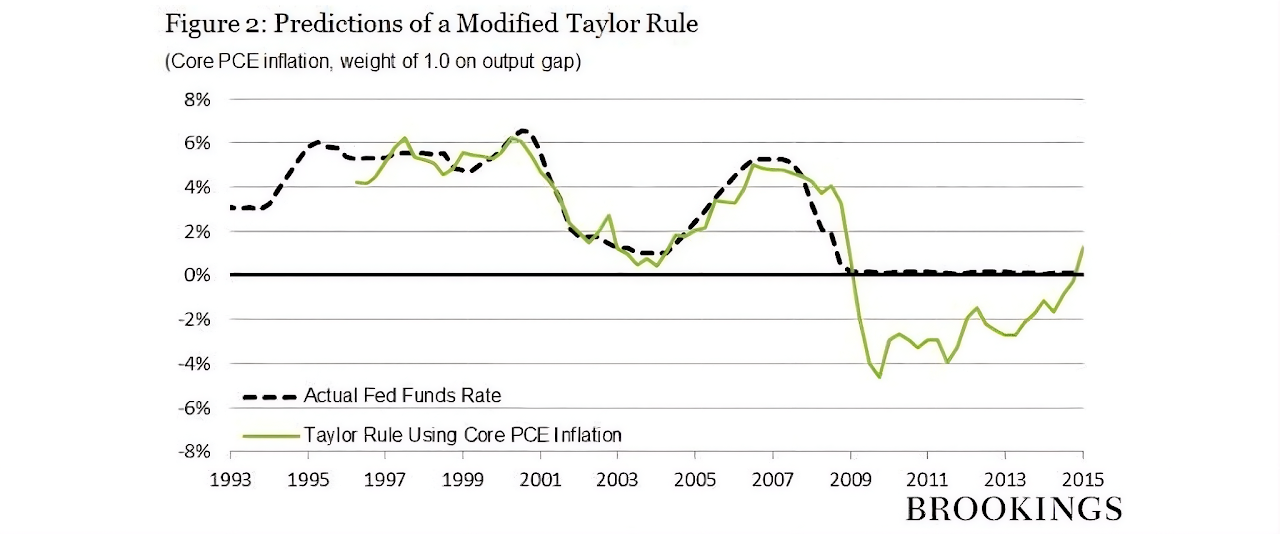
Figure 2: Comparison between actual federal funds rates and policy rates estimated by Bernanke’s updated rule throughout 1993-2015
This leads to his central conclusion: monetary policy should be systematic, not automatic. The rule provides the automatic framework, but the uniqueness of the crisis demanded a systematic, discretionary response, such as keeping rates at the ELB and implementing QE, measures that a rigid formula could never have prescribed. As Bernanke himself stated: "The simplicity of the Taylor rule disguises the complexity of the underlying judgments that FOMC members must continually make if they are to make good policy decisions".
4. Bernanke’s Updated Rule in a Brand New Environment
Following the GFC, central banks around the world embarked on an unprecedented era of unconventional monetary policy. Taylor himself labelled this period the "Global Great Deviation", arguing that the move away from predictable, rule-based approaches created a "strategy-free zone" where policy decisions became increasingly discretionary and difficult to anticipate.
This discretionary approach was characterized by:
- Quantitative Easing: Large-scale asset purchases that directly influenced long-term rates, bypassing the traditional short-rate channel. This measure has revealed to be drastically innovative for monetary policy, marking the final entrance of the latter into a brand new era.
- Forward Guidance: Central banks began communicating their intended future path of policy rates, effectively trying to manage expectations directly, thus affecting individuals and institutions’ spending and investment decisions. However, over the last years, this tool seems to have been left behind.
- Negative Interest Rates: In the euro area, the ECB pushed its deposit facility rate below zero, actually apporaching the ELB and testing the practical limits of monetary policy. The consequence was an extreme stimulus for financial intermediaries to lend and invest their excess liquidity
While these measures were supposedly necessary to relaunch the economy post-crisis, they made simple policy rules like the original Taylor equation less useful as a descriptive tool for actual central bank behavior. Yet, as Bernanke’s framework suggests, this does not mean the logic of rules was abandoned, only that the rules themselves needed to evolve to account for the new environment.
5. Backtesting the ECB (2015-2025): Taylor vs. Bernanke
To assess whether the European Central Bank has followed a rule-based approach in setting its policy rates over the last decade, we can apply the frameworks of both Taylor and Bernanke. Following Bernardini and Lin (2024), we focus on the Deposit Facility Rate (DFR) , which since 2014 has become the ECB’s key policy rate, the one on bank deposits held at the central bank and the primary instrument for signalling monetary policy positions. The DFR represents the floor of the ECB rates corridor, meaning that no bank or financial intermediary will lend to another at a lower rate.
5.1. The Empirical Evidence: A Different View of History
Applying the original 1993 Taylor rule to the ECB presents sudden challenges. The rule uses the GDP deflator and assumes a constant equilibrium real rate of 2%, while in the post-crisis environment, characterized by low growth and structural changes, the real equilibrium rate (r∗ ) has likely fallen significantly below 2%, as already mentioned.
Furthermore, as Bernardini and Lin (2024) highlight in their analysis of the ECB Survey of Monetary Analysts (SMA), using headline inflation in a Taylor Rule produces a systematically different prescription than using core inflation, which excludes volatile energy and food prices. The authors explicitly choose core HICP (i.e. Harmonised Index of Consumer Prices) inflation over headline, "because of its tendency to be a better indicator of future headline inflation than current headline itself and, therefore, to be more consistent with the mediumterm orientation of the monetary policy of the ECB".
Now, if we had to mechanically apply the original Taylor Rule using headline HICP inflation over the past decade, it would have likely prescribed a much faster and steeper normalization of rates than the ECB actually implemented, especially during the long period of negative rates and subdued inflation. The rule would have failed to account for the ELB constraint and the need for extraordinary accommodation, confirming Taylor’s own critique that central banks had deviated from his prescribed path. Finally, the rule would have consistently called for higher rates, misinterpreting inflationary pressures as a temporary factor rather than a radicated influence.
5.2. The Bernanke Rule Test
Bernanke’s updated framework, particularly the TPLT approach and his 2015 modified rule, offers a more accurate lens through which viewing ECB’s strategy. Just as Bernanke argued for using core PCE inflation and a higher output gap coefficient to accurately describe the Fed, Bernardini and Lin (2024) find that using core HICP inflation, but also the unemployment rate as a proxy for the output gap is a much more suitable solution.
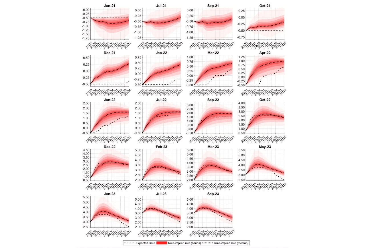
Figure 3: Comparison between analysts’ expectations and "bands" of rule-based rates, from which the median is evidenced as representative curve. These "bands" are linked to a "thick-modelling approach", consisting of 15,129 rules tested out, since countless deterministic rules exist and analysts might be using any of them.
5.3. Empirical Confirmation of the Theoretical Shift
The empirical evidence from Bernardini and Lin (2024) confirms the theoretical transition from Taylor’s original framework to Bernanke’s updated approach. In fact, their analysis of the ECB Survey of Monetary Analysts reveals a clear structural break that aligns quite precisely with the predictions of Bernanke’s philosophy. Before the summer of 2022, when the ECB’s policy rate remained constrained by the Effective Lower Bound and the Governing Council provided explicit forward guidance on the future path of rates, analysts’ expectations seemed pretty far away from conventional Taylor rule logic. During this period, the now acknowledged "strategyfree zone" of unconventional policy, the responsiveness of expected rates to changes in inflation and economic activity was anything but deterministically immediate. This reflects what Bernanke himself explained: at the ELB, the simple mechanical prescriptions of standard rules become unfeasible and policy must operate through alternative channels, such as the ones we have already mentioned.
However, once the ECB moved decisively away from the ELB in July 2022 and discontinued the exploitation of forward guidance, a remarkable re-anchoring occurred, as easily noticeable in Figure 3. Analysts’ expectations of the future path of the DFR became closely aligned with the prescriptions of simple monetary policy rules, but crucially, not Taylor’s original specification. Instead, the rule that best described these expectations employed precisely the refinements Bernanke had brought on the table: core inflation rather than headline and unemployment rate, seen as a better measure of economic cycles, rather than the output gap derived from potential GDP estimates.
Undoubtedly, these findings carry deep theoretical significance. In fact, they suggest that while central banks may be forced into discretion during crises, following the "systematic, not automatic" approach that Bernanke underlined, the logic of rules never truly disappears. It merely hides, waiting to reassert itself once extraordinary circumstances begin to vanish.
5.4. The Shadow Rate and TPLT Interpretations
The qualitative pattern observed in analysts’ expectations before and after July 2022 can also be interpreted through the lens of Bernanke’s two specific proposals. The period of subdued policy responsiveness at the ELB is consistent with a shadow rate framework: during the ELB years, analysts understood that the actual policy rate was constrained, but they calibrated their expectations based on a notional shadow rate that would eventually guide the exit from the bound. When the shadow rate finally rose above the ELB threshold, expectations quickly re-anchored to conventional rule parameters.
Similarly, the post-2022 alignment with core inflation expectations reflects the logic of Temporary Price Level Targeting. Throughout the tightening cycle, the ECB consistently emphasized that the cumulative shortfall of inflation from the 2% target during the preceding years would not be ignored. This is precisely the TPLT philosophy: ensuring that past inflation, below target for several years, is compensated through a sustained commitment to the target itself, even at the cost of allowing inflation to run moderately above it for a period. The fact that analysts’ expectations incorporated this logic confirms that Bernanke’s framework not only describes how central banks should behave, but also how sophisticated market participants expect them to behave.
6. Conclusion
The journey from Taylor’s original 1993 Rule to Bernanke’s updated proposals mirrors the evolution of monetary policy itself. The original Taylor Rule provided a foundational framework, however it proved to be insufficient in environments different from NICE, characterized by crises and consequent necessary discretionary strategies with extremely low rates and alternative measures. On the other hand, Bernanke’s adaptations managed to offer a way more complete toolkit for both policymakers and market analysts, by refining the measurement of key inputs and acknowledging the constraints of the ELB. Systematic, not automatic has proved to be the most applicable school of thought.
However, the matter changes interestingly in normal times. When the fog of crisis lifts, the logic of rules reasserts itself and expectations of those who watch central banks most closely fall back into the familiar patterns that Taylor first identified over three decades ago, now refined and updated by Bernanke for a new era of monetary policy, where nothing is taken for granted, but everything lays on solid foundations, sometimes hidden, but generally pretty robust.
References
[1] Ben S. Bernanke. The taylor rule: A benchmark for monetary policy?, April 2015.
[2] Ben S. Bernanke. Monetary policy in a low interest rate world: Comment. Brookings Papers on Economic Activity, pages 335–342, 2017.
[3] Ben S. Bernanke. Monetary policy in a new era. In Rethinking Monetary Policy in a New Normal. Peterson Institute for International Economics, Washington, DC, 2017.
[4] Marco Bernardini and Alessandro Lin. Out of the elb: Expected ecb policy rates and the taylor rule. Technical Report 815, Banca d’Italia, Rome, 2023.
[5] Marco Bernardini and Alessandro Lin. Out of the elb: Expected ecb policy rates and the taylor rule. Economics Letters, 235:111546, 2024.
[6] James Hebden and David López-Salido. From taylor’s rule to bernanke’s temporary price level targeting. Technical Report 2018-051, Board of Governors of the Federal Reserve System, Washington, DC, 2018.
[7] John B. Taylor. Discretion versus policy rules in practice. Carnegie-Rochester Conference Series on Public Policy, 39(1):195–214, 1993.